Since I have been intensifying my efforts in the generative art space, I’ve been making more and more use of the illustrious Perlin noise algorithm.
You might have seen me mentioning it on in the description of one of my Instagram posts, or in my previous newsletter. And maybe you read it and thought: ‘What the heck is this guy talking about?’
Well… I’m here to explain that now. And not only will I explain it to you. I will also explain it to myself :) I’ll be doing research into the concept of Perlin noise, its history, background, and implementations. So without further ado, let’s see what we are talking about!
What is Perlin noise?
Perlin noise is a type of pseudo-randomness that was initially developed to create procedural texture for 3D models in computer graphics. The model is so perfect for this because it does not generate completely random values. Instead, it creates pseudo-random values.
You see, complete randomness is hectic and chaotic. It's something that does not appear to be very natural, because for some reason nature always seems to appear in patterns to the human eye. It does not matter if we understand those patterns or if we can truly notice them, there always seems to be a certain cohesion in nature that we intuitively catch onto.
So when computer scientist Ken Perlin was working on Disney's computer-animated sci-fi motion picture Tron in 1983, he decided that he needed a sophisticated algorithm that could mimic that sense of organic randomness that we see in nature. And that's when he developed what is now known as Perlin noise.
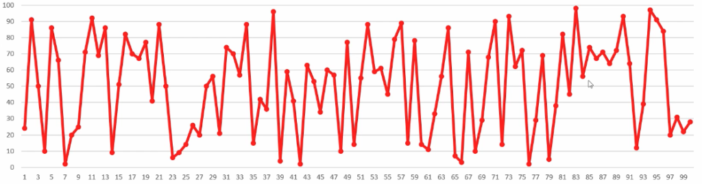
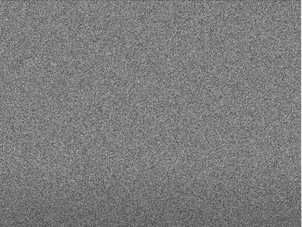
Graph #1 - A graph of completely random numbers. Very ugly and chaotic.
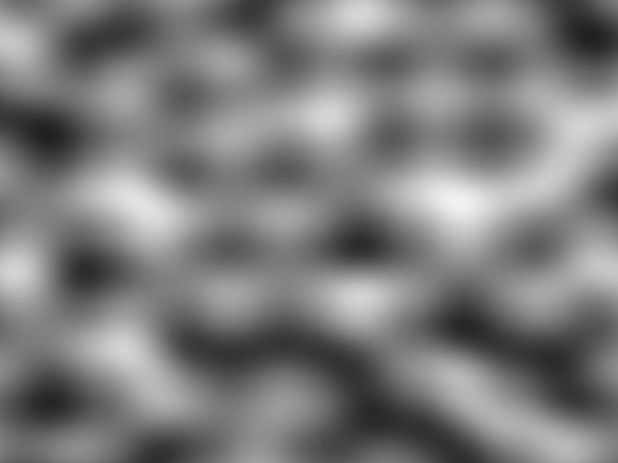
To illustrate what Perlin noise is, you should have a look at the graph above. It's a graph of completely random numbers. It looks chaotic and not very nice. Now look at the graph underneath here. It's the same amount of points, in the same range. But instead of chaos, there seems to be an organic relation between the points. It does not exactly look like a clear pattern, but you can see that the points relate to each other in some sort of way.
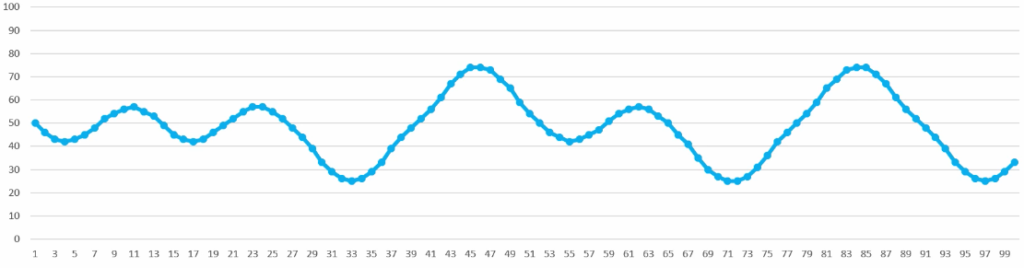
A graph of pseudo-random numbers (Perlin noise). Very smooth and pleasant on the eye.
So that’s what Perlin noise is in a nutshell. It’s a model that can generate pseudo-random numbers. Numbers that are random, but seem to relate to each other in some sort of fashion. And that concept of those pseudo-random numbers is very powerful. Especially when we are talking about natural things. Think of landscapes, the organic growth of plants, or the movement of clouds. All those examples can seem random to the human eye, but they all seem to possess some sort of natural, organic sequence.
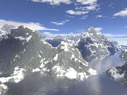
A virtual landscape generated using Perlin noise (via Wikiwand)
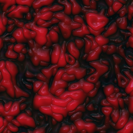
An organic surface generated with Perlin noise (via Wikiwand)
Ken Perlin’s Academy Award
You can imagine what a terrific invention this algorithm was and what an impact it left in the field of computer graphics. It will then not surprise you that in 1997, Ken Perlin was awarded an Academy Award (Oscar) for his contribution to the field for his efforts to create the computer-simulated world of the 1983 Tron movie. And still to this day, it's a very popular algorithm that is being used in the generative art space and in computer graphics.

Still from the 1983 motion picture Tron (via Wiener Zeitung)
How does it work?
This is where it gets interesting. It is easy to use the Perlin noise model in generative art without really understanding how it works. It’s basically a built-in function in a lot of libraries that you can freely use. You give it input and the function provides you with some interesting output. But it’s a black box model. You don’t know what it does if you don’t dig into it. That’s why I thought it might be interesting to pop open the hood of this machine and have a look at the mechanics :)
First, it's important to know that you can use Perlin noise to create 1-dimensional objects (e.g. a line), 2-dimensional objects (e.g. a grid), or 3-dimensional objects (e.g. a ball).
1D Perlin Noise
2D Perlin Noise
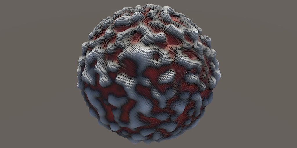
3D Perlin Noise (via Catlike Coding)
To explain the concept of Perlin noise, we'll focus on 2D Perlin noise. I am going to follow much of this tutorial by Fataho that I found online. It's by far the best tutorial I could find on this topic.
The goal for this example is to create a 2D grid of pixels of which the colours are established based on Perlin noise. In the pictures below you'll see what I mean. Instead of giving every pixel a completely random value (picture #1), we give every pixel a pseudo-random value (picture #2). This means that it's still sort of random, but it is also influenced by the values that surround the pixel. That's how you get this natural, organic feeling to it.
Picture #1 a grid of completely random coloured pixels
Picture #2: a grid of pseudo-randomly coloured pixels (2D Perlin noise)
Alright, now that we have established what our goal is, we can finally start implementing it.
Firstly, we start off by creating a grid of pixels.
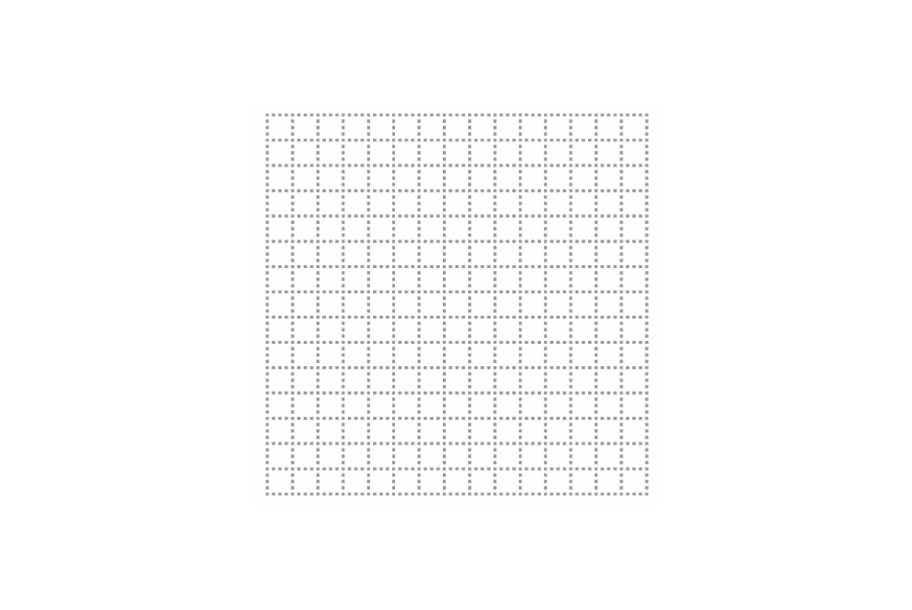
A grid of pixels (conceptual)
After that, we divide the grid into sections. We place an imaginary second grid - with larger squares - on top of the first grid.
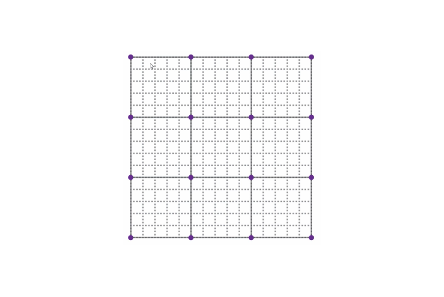
Imaginary grid with larger squares on top of the original grid.
The points where lines of the second grid intersect - as indicated by the purple dots - are going to be important now. These dots will be the starting points of some imaginary vectors that we will draw.
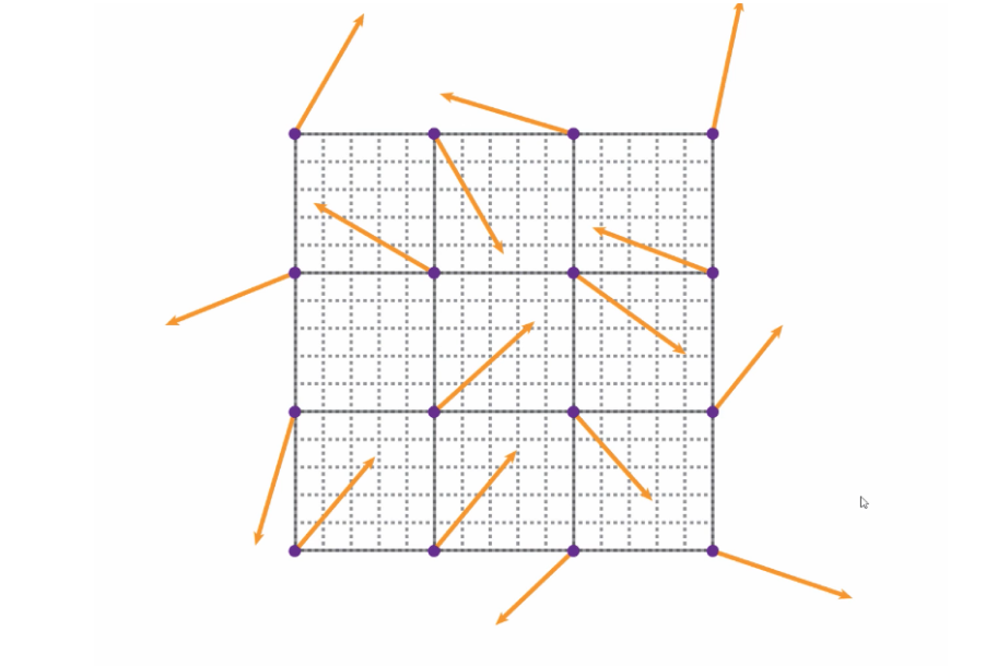
Random vectors
In the image above, the vectors all have the same length but the angles are completely random. In order to simplify the Perlin noise algorithm we will limit the number of angles that can be used for the vectors. They will still be randomly selected, but instead of having 360 degrees to choose from, we will limit the number of options to four. This choice is purely done for performance's sake. It's cheaper and faster to work with only four options.

The selected vectors.
There are people that use all eight vectors from this diagram, but for simplicity's sake, we will only use the diagonal ones. These are the vectors:
-
(-1, 1)
-
(1, 1)
-
(1, -1)
-
(-1, -1)
That means we have an array of four different vectors. The next step is then to randomly asign one of these vectors to every purple dot.
A subsection of the grid, with vectors.
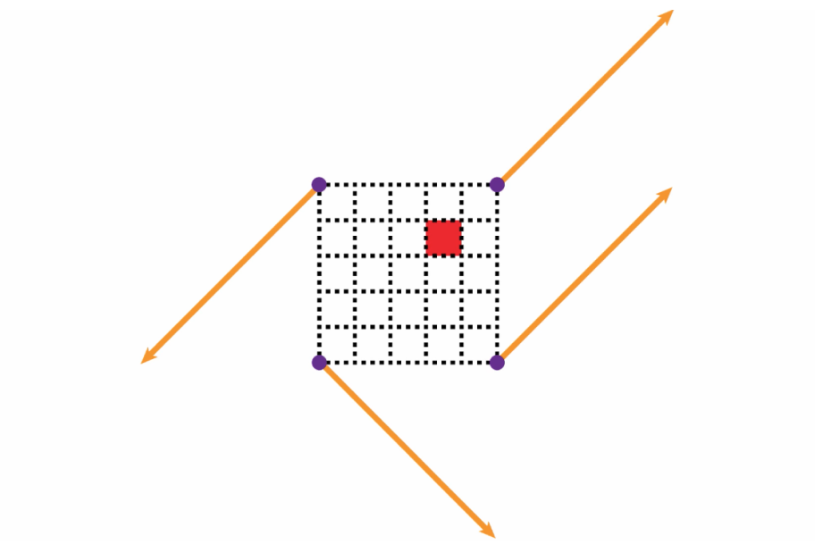
With the vectors drawn, we now have all the tools in place to calculate the colour value of every individual pixel of the original, underlying grid. For this example, we'll just focus on the red pixel, but the process will be the same for all other pixels.
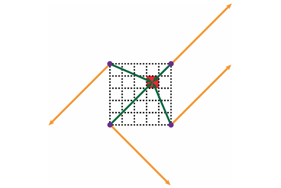
Random vectors (orange) and distance vectors (green).
The first step will be to draw four distance vectors from the purple points to our target pixel. For this example, we can use the dimensions of the image below.
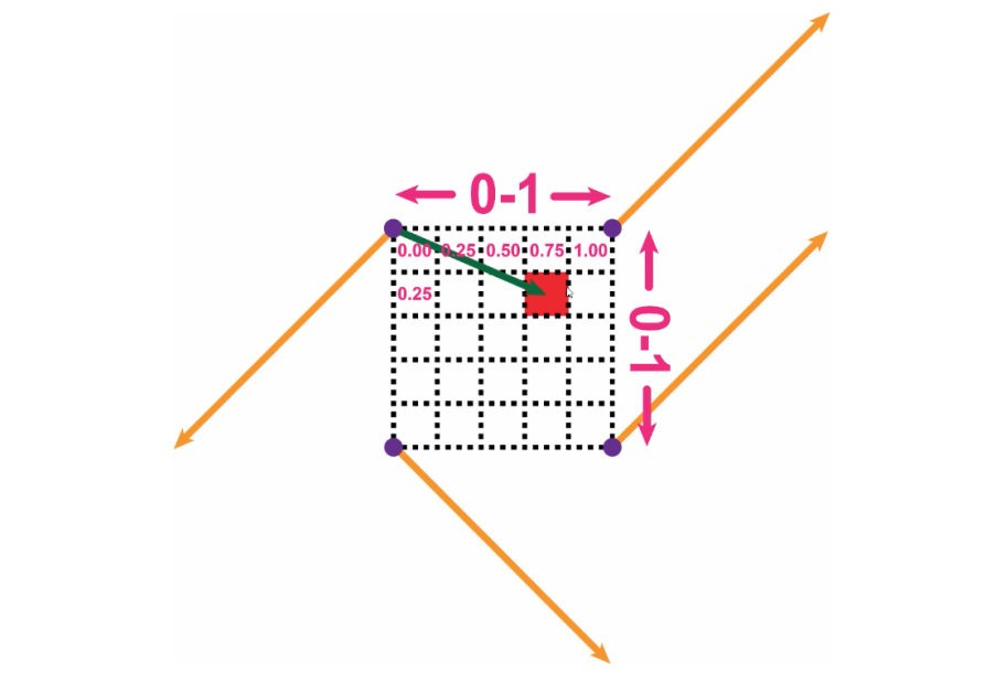
Calculating the distance vectors.
Following this method will give us four distance vectors below:
-
(0.75, 0.25)
-
(-0.25, 0.25)
-
(-0.25, -0.75)
-
(0.75, -0.75)
Once every purple dot has an orange and a green vector, we will calculate the dot product of both of these vectors. To calculate the dot product, we simply add up the product of the x-components of both vectors and the y-component of both vectors. See the calculation below for the first purple dot.
D1 = G(-1, 1) * D(0.75, 0.25)

D1 = -1 * 0.75 + 1 * 0.25

D1 = -0.75 + 0.25 = -0.5
By doing so, we end up with only one value for each purple dot (relative to our target pixel). Now that we have established these numbers for each purple dot, we can calculate the value of our target pixel. We do this by applying bilinear interpolation. First, we interpolate between DotA and DotB (and between DotC and DotD) as indicated by the blue lines. After we've done that, we interpolate between those two values (green line) to find the value of our target pixel.
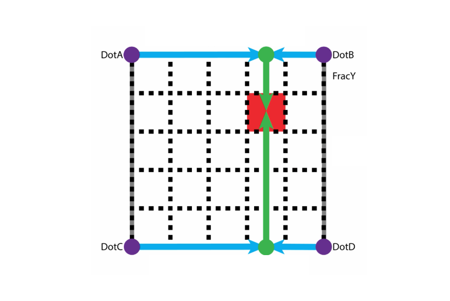
Interpolating to find the value of our target pixel.
Simply put, interpolation is trying to calculate the coordinates of a point that falls between two other points. So to calculate the point between DotA and DotB (or X0Y0 and X1Y1 in the graph below), we first calculate the slope between X0Y0 and X1Y1. And because the relation between all the points is linear, we can then use that slope value to calculate point XY. The formula below shows the basic idea behind this calculation (assuming you know X0Y0, X1Y1, and either X or Y of your target point).

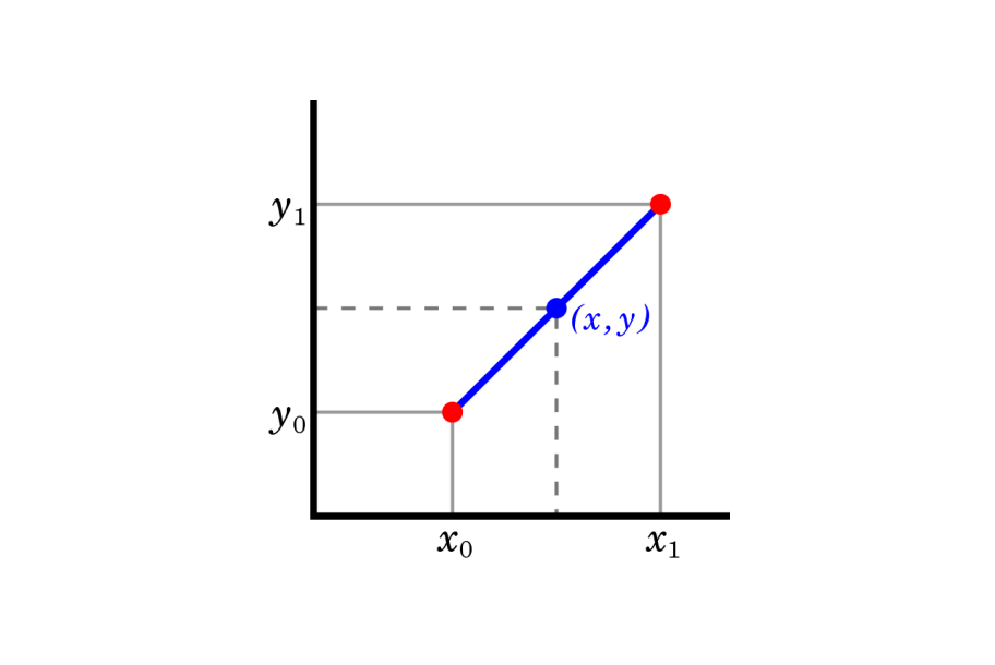
Linear interpolation (via Wikipedia)
And that is basically it.
To calculate the value of every pixel, you simply repeat this process. Because the colour of every pixel is based on the random vectors (orange) and the distance vectors (green), you can see that all pixels in between the four purple dots will be somewhat similar in colour. There is only a minimal difference that is caused by the difference in the distance vector. This difference will already cause an interesting-looking grid of pixels between the four purple dots. But then imagine the selection of pixels between the next four purple dots. They will have two purple dots in common with the selection in the image above, but they will also have two other purple dots bordering them. This means that the value of the pixels in this neighbouring selection will be influenced by both two similar vectors and two different vectors. This will ensure that the values of this neighbouring selection will never be too far off the first selection.
You can see how this chain-like behaviour between the selection of pixels now causes the colour-values of the pixels to display an organic relationship that is very pleasing to the eye.
I hope that this explanation has provided some clarity into what Perlin noise is and how it works. A big shout out to Fataho for the great tutorial in which he explains the mathematics of Perlin noise. If you are interested I recommend watching his video tutorial.